Table of Contents
Linear Regression
Linear Regression is a type of Regression Analysis where we fit a set of data points to a straight line.
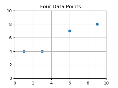
For example, here are four (x,y) data points which appear roughly in the shape of a straight line.

| x | y |
|---|---|
| 1 | 4 |
| 3 | 4 |
| 6 | 7 |
| 9 | 8 |
Trial and Error
 How do we find the equation for the line that best fits these four points. One way is trial and error.
In this graph we made three attempts, and that third line comes pretty close, but now we need to be more rigorous and more mathematically certain.
Least Squares
Predictor Function
Write the linear equation as a function of $x$. $$f(x) = ax + b$$ This is the predictor function. $f(x)$ gives the predicted value of $y$.
Error
Compare the predicted value to the actual value of y by subtracting. $$f(x) - y$$ This gives us the error of the predictor function for each data point. The error is also sometimes called the residual.
Squared Error
Square the error to make it more intense. $$(f(x) - y)²$$ The squared error.
Sum of Squared Error
Sum the squared error for all $n$ data points. $$\sum_{i=1}^n (f(x_i) - y_i)$$ The sum of the squared errors.
Vectorized
Now let's set up to calculate the least squares for all of the data points in one go using Matrix Math.
Rewrite the predictor function like this. $$f(X,θ) = \theta_0 x_0 + θ_1 x_1$$
where
$θ$ is a vector containing the values for $a$ and $b$ (in reverse order),
$X$ is a matrix containing the $x$ data points, prefixed with a column of ones, and
$y$ is a vector containing the $y$ data points, like this:
$$\theta=\begin{bmatrix}2\\.8\end{bmatrix}\hspace{30pt}x=\begin{bmatrix}1&1\\1&3\\1&6\\1&9\end{bmatrix}\hspace{30pt}y=\begin{bmatrix}4\\4\\7\\8\end{bmatrix}$$
Now the predictor function simplifies to $f(X,θ) = θ<sup>T</sup>X$ using element-wise matrix multiplication, and
Sum of Squared Errors = $∑(((θ X) - y)^2)$
In Octave:
Sum_of_Squared_Errors = sum(theta' .* x,2)
This equation is generalized to use any number of input values, by expanding $θ$ and $X$.
Least Squares
Now we have a single number to represent the accuracy of the predictor function. We can calculate the sum of the squared errors for different predictor functions, and the one with the smallest value, the least squares, is the best predictor.
Optimize
 Our goal is to find the optimal $θ$, the one that gives us the least squares.
We will use three systematic methods based on least squares.
- Brute Force (blue)
- Normal Equation (orange)
- Gradient Descent (green)
Normal Equation
Applying Differential Calculus to minimize the Sum of Squared Errors, we come up with this formula:
$$\theta = \left ( X^T X \right )^{-1}X^T y$$
But that was much too easy, so let's continue on with the Gradient Descent method.
Gradient Descent
We can use gradient descent to minimize the cost function. That is to say, we use gradient descent to find the optimal values of theta.
Gradient Descent is an algorithm for finding the optimal theta.
Gradient Descent is an algorithm for finding the optimal theta.
We run the predictor function many times, each time with a different value of theta. It is set up mathematically so that each iteration gets a little closer to the optimal theta.
Iterative Steps
Here is the pseudo code for gradient descent.
set number//of//iterations
set alpha α
set starting θ
For (1 to number_of_iterations)
    Calculate the cost function J(θ)
    Calculate the gradient g(θ)
    Subtract the gradient from θ
end loop
Hypothesis
We can rename the predictor function to the hypothesis. So $f(X,θ)$ becomes $h_θ (X)$. With each iteration, we test a new and improved hypothesis.
Cost Function
The Cost Function is another name for the Sum of Squared Errors formula. Or it can be a modified version of the Sum of Squared Errors formula.
Andrew Ng multiplies the Squared Errors formula by $1/2m$, where m is the number of data points. He says this makes the math work out better.
$$J(\theta ) = \left ( \frac{1}{2m} \right )\sum \left ( h_\theta (x) - y)^2 \right )$$ where $m$ = the number of data points
In Octave, it looks like this:
J = (1/(2*m)) * sum((sum(theta' .* X,2) - y).^2);
Gradient
Like the derivative, the gradient represents the slope of the tangent of the graph of the function. More precisely, the gradient points in the direction of the greatest rate of increase of the function, and its magnitude is the slope of the graph in that direction.
But the way Andrew Ng is doing it, it's not a derivative function, it's just a percentage of the error times the X factor.
Also, the Andrew Ng course led me to believe that alpha is part of the gradient formula. But it is not. It is again taking a percentage of the gradient to apply to the new theta.
$$g(θ) = α(\frac{∂}{∂θ}) J(θ)$$
where
$α$ = learning rate, and
$\frac{∂}{∂θ}$ = partial derivative of $J(θ)$ with respect to $θ$
Expanded, it looks like this: $$g(θ) = α \frac{∂}{∂θ} (\frac{1}{2m})\sum_{i=1}^m(hθ(x_i)−y_i)^2$$
where
$α$ = learning rate, and
$\frac{∂}{∂θ} J(θ₀,θ₁) = $ derivative
$\frac{∂}{∂θ} J(θ₀,θ₁) = $ partial derivative (same thing)
$$\frac{∂}{∂θ} = 1/m = 1/2$$
In Octave
gradient = alpha * (1/(2*m)) * sum(((sum(theta' .* X,2) - y).*2) .* X);
Normalized Data
Variations
References
- Source: Andrew Ng, Coursera Machine Language course, week 2
